#30DMC_15Nov_MyData

15 November. Data: my data.

“Map something personal. Map data from your own life—this could be places you’ve traveled, your daily routine, or any other personal touch.”

1. Package Installation and Loading

# Define the packages to be used
packages <- c("tidyverse", "sf", "osmdata",
              "geojsonR", "httr2", "stringr",
              "lubridate", "magick", "magrittr",
              "grid", "extrafont")

# Function to check if packages are installed and load them
load_packages <- function(pkgs) {
  # Check for missing packages
  missing_pkgs <- pkgs[!(pkgs %in% installed.packages()[, "Package"])]
  
  # Install missing packages
  if (length(missing_pkgs)) {
    install.packages(missing_pkgs)
  }
  
  # Load all packages
  lapply(pkgs, library, character.only = TRUE)
}

# Load the packages
load_packages(packages)
loadfonts(device = "postscript")

2. Import personal data, city backgrounds & Rbanism logo

# Personal data
# https://www.google.com/maps/d/edit?mid=1u_XNZO2eSg8vmpIPjjkHy2nDyPEiuhGa&usp=sharing
mydata <- read_csv("MyData.csv") %>%
  mutate(long =  word(word(word(geometry, 2, sep="\\("), 1,  sep="\\)"), 1, sep="\\ "),
         lat =  word(word(word(geometry, 2, sep="\\("), 1,  sep="\\)"), 2, sep="\\ "),
         date = dmy(time))

Rows: 45 Columns: 2
── Column specification ────────────────────────────────────────────────────────
Delimiter: ","
chr (2): geometry, time

ℹ Use `spec()` to retrieve the full column specification for this data.
ℹ Specify the column types or set `show_col_types = FALSE` to quiet this message.

# Direction de l'Urbanisme - Ville de Paris, Opendata Paris, Open Database License (ODbL) https://opendata.paris.fr/explore/dataset/quartier_paris/export/?disjunctive.c_ar&location=12,48.85889,2.34692&basemap=jawg.streets
paris_WGS84 <- st_read("quartier_paris.geojson") 

Reading layer `quartier_paris' from data source 
  `/Users/ccottineau/GitHub/30DayMapChallenge2024/15Nov_MyData/quartier_paris.geojson' 
  using driver `GeoJSON'
Simple feature collection with 80 features and 11 fields
Geometry type: POLYGON
Dimension:     XY
Bounding box:  xmin: 2.224078 ymin: 48.81558 xmax: 2.469761 ymax: 48.90216
Geodetic CRS:  WGS 84

paris_crs <- 27572

paris_metric <- paris_WGS84 %>%
  st_transform(.,crs=paris_crs)

# Greater London Authority, Ordnance Survey data with © Crown copyright https://data.london.gov.uk/dataset/statistical-gis-boundary-files-london
london_metric <- st_read("London_Ward.shp") 

Reading layer `London_Ward' from data source 
  `/Users/ccottineau/GitHub/30DayMapChallenge2024/15Nov_MyData/London_Ward.shp' 
  using driver `ESRI Shapefile'
Simple feature collection with 657 features and 6 fields
Geometry type: POLYGON
Dimension:     XY
Bounding box:  xmin: 503568.2 ymin: 155850.8 xmax: 561957.5 ymax: 200933.9
Projected CRS: OSGB36 / British National Grid

london_crs <- 27700
  
london_WGS84 <- london_metric  %>%
  st_transform(.,crs=4326)

# Download Rbanism logo
rbanism_logo <- image_read('https://rbanism.org/assets/imgs/about/vi_l.jpg')

3. One function to filter, crop and map data

city_flash_map <- function(city){

if(city == "Paris"){
city_metric <- paris_metric
city_WGS84 <- paris_WGS84
city_crs <- paris_crs
source <- "Direction de l'Urbanisme - Ville de Paris, Opendata Paris ODbL"
}

if(city == "London"){
city_metric <- london_metric
city_WGS84 <- london_WGS84
city_crs <- london_crs
source <- "Greater London Authority, Ordnance Survey w/ © Crown copyright"
}
  
bbWGS <- sf::st_bbox(city_WGS84)
  
### Filter my data to city

mydata_sf <- st_as_sf(mydata, coords = c("long","lat")) %>%
  st_set_crs(4326) %>%
  st_transform(.,crs=city_crs) %>% 
  st_intersection(city_metric, .) 

mydata_sf <- mydata_sf %>%
  mutate(days = as.numeric(max(mydata_sf$date) - date))

### Import OSM data
# Metro
x <- opq(bbox = bbWGS) %>%
   add_osm_feature(key = 'railway', value = "subway") %>%
    osmdata_sf() 

# Waterways
y <- opq(bbox = bbWGS) %>%
   add_osm_feature(key = 'waterway') %>%
    osmdata_sf() 

# Green spaces
z <- opq(bbox = bbWGS) %>%
   add_osm_feature(key = 'leisure', value="park") %>%
    osmdata_sf() 

### Crop OSM features to city extent
metrolines <- x$osm_lines %>%
  st_transform(.,crs=city_crs) %>%
  st_intersection(city_metric, .)

water <- y$osm_lines %>%
  st_transform(.,crs=city_crs) %>%
  st_intersection(city_metric, .) %>%
  filter(waterway %in% c("canal", "river"))

green <- z$osm_polygons %>%
  st_transform(.,crs=city_crs) %>%
  st_intersection(city_metric, .)


## Plot the result
ggplot() +
   geom_sf(data = city_metric, fill=alpha("grey", 0.8), colour = "white") +
  geom_sf(data = water, colour=alpha("#93278F",0.7), aes(linewidth=waterway)) +
  scale_discrete_manual("linewidth", values = c(1,2))+
 # geom_sf(data = metrolines, aes(colour=ref)) +
  geom_sf(data = green, fill="#00A99D", colour = "white", linewidth = 0) +
  geom_sf(data = mydata_sf, aes(colour = days), size=3) +
  coord_sf(datum = st_crs(city_crs)) +
  scale_colour_gradient(low = "white", high = "#F7931E",
                      na.value = NA, name="# Days since \n earliest flash") +
  ggtitle(paste0("15Nov. My Data \n",
                 city, " flashes during the first COVID lockdown")) +
    ylab("")+
  xlab(paste0("#30DayMapChallenge. Clémentine Cottineau-Mugadza, 2024. Personal data.\n Map background: ", source, ".")) +
  guides(linewidth  = "none") +
  theme_minimal() +
  theme(axis.text=element_text(size=6, family="Courier"),
       plot.title=element_text(size=12, family="Courier"),
        axis.title=element_text(size=8, family="Courier"),
       legend.text=element_text(size=8, family="Courier"),
       legend.title=element_text(size=10, family="Courier")) 

}

4. Pick a city and make a map

Paris

city_flash_map("Paris") 
grid.raster(rbanism_logo,
            x = 0.9, y=0.9,
            width = unit(100, "points"))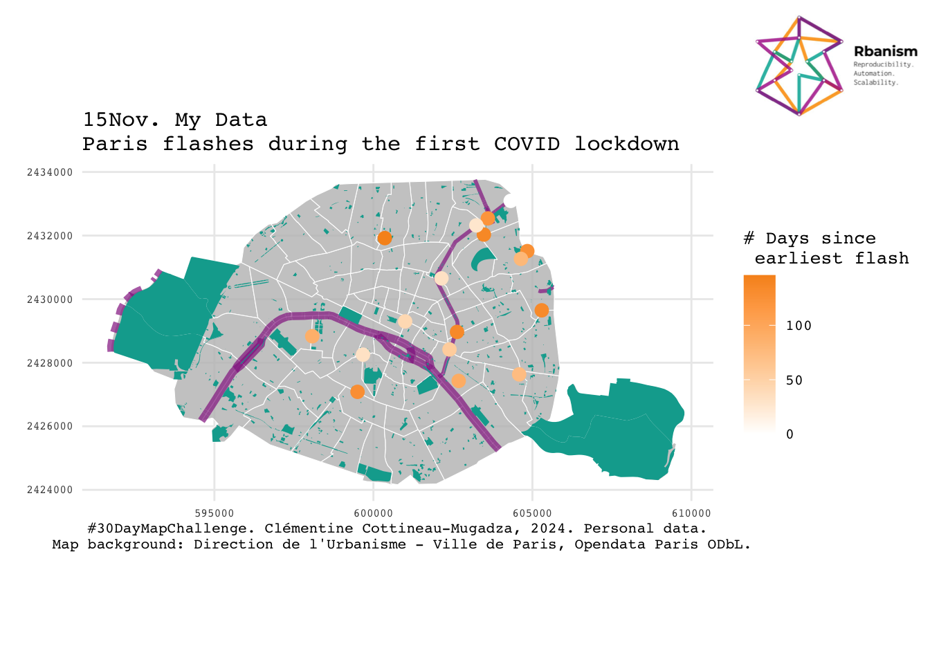

  ggsave(filename = "Paris.png",
         width = 8, height = 8, dpi = 300)

London

city_flash_map("London") 
grid.raster(rbanism_logo,
            x = 0.9, y=0.9,
            width = unit(100, "points"))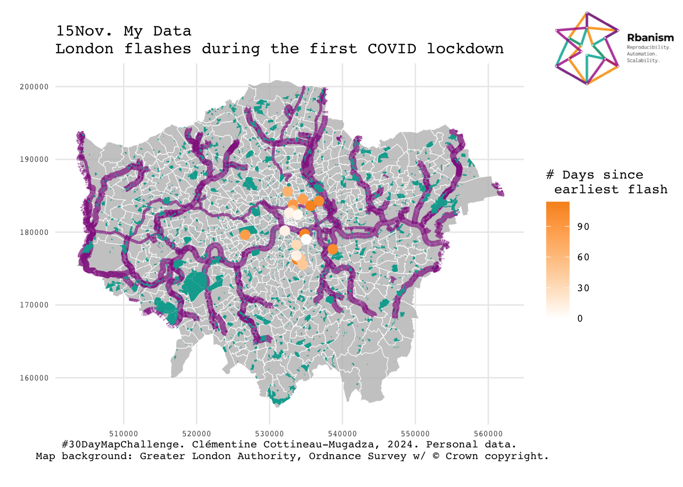

  ggsave(filename = "London.png",
         width = 8, height = 8, dpi = 300)